Hi everyone!!
I finaly got some time to work on the lab.
For
Section 1 by hand
1) data: 67.3, 61.8, 63.7, 62.4, 65.6,
66.2, 69.8, 63.9, 45.8, 78, 32, 68.0
a) mean: 62.04
data
/ number of occurrences = mean
(67.3
+ 61.8 + 63.7 + 62.4 + 65.6 + 66.2 + 69.8 + 63.9 + 45.8 + 78 + 32 + 68.0) / 12 =
mean
b) variance: 143.70
data
– mean = (x) squared = y
67.3
- 62.04 = (5.26) squared = 27.6676
61.8
- 62.04 = (-0.24) squared = 0.0576
63.7
- 62.04 = (1.66) squared = 2.7556
62.4
- 62.04 = (0.36) squared = 0.1296
65.6
- 62.04 = (3.56) squared = 12.6736
66.2
- 62.04 = (4.16) squared = 17.3056
69.8
- 62.04 = (7.76) squared = 60.2176
63.9
- 62.04 = (1.86) squared = 3.4596
45.8
- 62.04 = (-16.24) squared = 263.7376
78.0
- 62.04 = (15.96) squared = 254.7216
32.0
- 62.04 = (-30.04) squared = 902.4016
68.0
- 62.04 = (5.96) squared = 35.5216
(y1
+ y2 +
y3 + y4 + y5 +
y6 + y7 + y8 +
y9 + y10 + y11 +
y12) / 12 = variance
c) standard deviation: 11.99
Standard deviation = square root (variance)
For
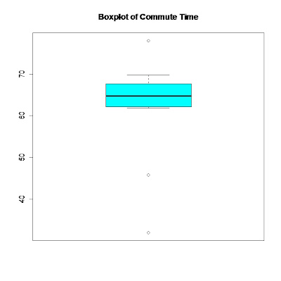
Section 2 of the lab using "R"
Using “R”
>
commute = c(67.3, 61.8, 63.7, 62.4, 65.6, 66.2, 69.8, 63.9, 45.8, 78, 32, 68.0)
>
commute
[1] 67.3 61.8 63.7 62.4 65.6 66.2 69.8 63.9
45.8 78.0 32.0 68.0
>
mean (commute)
[1]
62.04167
>
sd (commute)
[1]
11.9873
>
var (commute)
[1]
143.6954
INPUT into “R”….
>
hist(commute, xlab ="Commute Time", main ="Histogram of Commute
Time", col = 3, breaks = 6)
INPUT into “R”….
>
boxplot(commute, main = "Boxplot of Commute Time", col = 5)
INPUT into “R”….
>
qqnorm(commute, main = "Commute Time")
>
qqline(commute)
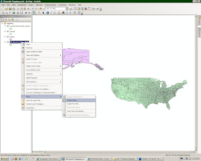
For Section 3 of the lab using ArcGIS...
-I started out inputing the earthquake data, and reprojecting using....
Data Mangment Tools
>Projected and Transfomations
>Feature
> Project
Project Coordinate System
>Continential
>North America
>Noth America Equal Area Conic.prj OR Alaka Albers Equal Area Conic.prj...
-below I found the mean center/meadian center using the following tool in "tool box"
Spatial Statistic Tools
>Measuring Geographic Distrubution
>Mean Center
OR
>Median Center
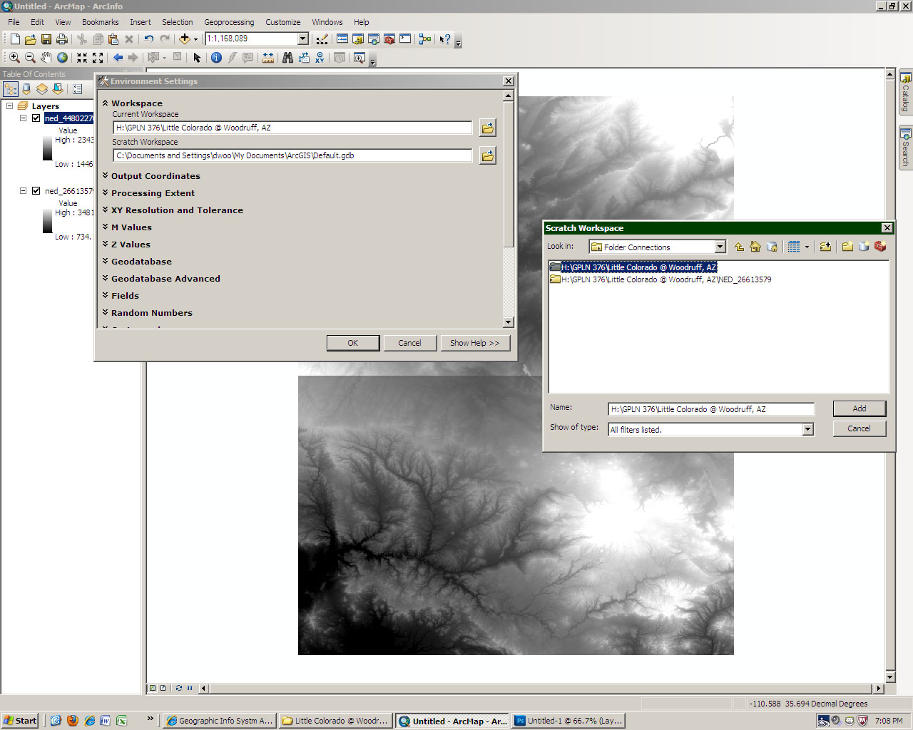
-below I used the Geostatistical Analyst Tool, first you had to go to...
Customerize
>Extenision
>Geostatistical Analyst
THEN
Customerize
>toolbars
>Geostatistical Analyst
WHEN the tool bar is present click on the...
Geostatistical Analyst
>Explore Data
>Historgram
-below I used the Geostatistical Analyst Tool, first you had to go to...
Customerize
>Extenision
>Geostatistical Analyst
THEN
Customerize
>toolbars
>Geostatistical Analyst
WHEN the tool bar is present click on the...
Geostatistical Analyst
>Explore Data
>QQ plot
-below I found the mean center/meadian center using the following tool in "tool box"
Spatial Statistic Tools
>Measuring Geographic Distrubution
>Directional Distrubution
-below I used the Geostatistical Analyst Tool, first you had to go to...
Customerize
>Extenision
>Geostatistical Analyst
THEN
Customerize
>toolbars
>Geostatistical Analyst
WHEN the tool bar is present click on the...
Geostatistical Analyst
>Explore Data
>Voronoi Map